
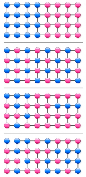
 Let us consider the four 32-node graphs appearing in the figure to the left. We would like to regard these graphs as representing the distributions of some quantities of interest. More specifically, for each graph, there exists a quantity whose value is defined at each node, and the value of this quantity characterizing each node is independent of time.
For example, in the case of a market survey carried out by a social networking service, this quantity could represent the level of interest shown by each user for a particular product, and in the case of Web searches, it could be a binary quantity indicating whether a given search contained some particular word of interest. The values of these quantities at the nodes are indicated by the colors of the corresponding dots. (The quantities could be defined as continuous variables, with dot colors varying continuously between pure red ![]() and pure blue
and pure blue ![]() , but here, we consider only the case of binary quantities.)
, but here, we consider only the case of binary quantities.)
The first three graphs we consider are square lattices, while the fourth is a square lattice with several links missing. In the third and fourth graphs, the distributions of blue ![]() and red
and red ![]() dots are identical.
dots are identical.
With the small graphs considered here, obviously, one can visually easily distinguish graphs with different link structures or distributions of quantity values. However, if the number of nodes becomes large, it becomes difficult to simultaneously grasp the link structure and the distribution of quantity values. Now, let us consider a random walker that wanders from node to node (over existing links) on such a graph.
We can form a random time series consisting of the sequence of values of the quantity at each node visited along this walk. Then, let us consider the question of whether we could simultaneously characterize the link structure and the distribution of values of the quantity from the large deviation statistics of the fluctuations of this time series.
In the case of the first graph, between the two extreme time series in which 0 is repeated forever and 1 is repeated forever, there are time series in which 0 and 1 appear in random successions. For this graph, the rate function for the value of the quantity is a smooth, downward convex function defined on the interval from 0 and 1, realizing its minimum of 0 at the long-time average, 1/2.
In the case of the second graph, no matter what random walk is realized, the resulting time series is 0,1,0,1… Hence, there are no fluctuations. Here, the rate function is defined at a single point, 1/2, where it takes the value 0. It is interesting that although the structures of the graphs in these first two cases are identical, the difference between the distributions of the quantity in the two cases results in rate functions of such different types.
The third and fourth graphs represent the opposite situation. Here, although the distributions of the quantity are identical, the link structures differ. This too results in different rate functions in the two cases.
Next, let us consider the two small graphs to the left.
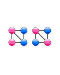 Both of these are 4-node graphs that differ only slightly from complete graphs, due to the lack of a single diagonal link. Their link structures are identical. However, the distributions of the quantity differ for the two, and as a result, the properties of the fluctuations exhibited by time series obtained from them will also differ. Now, let us consider all eight nodes of these two graphs together, and place very weak, non-directional links between every pair therein.
We refer to the strength of these links as ε and the strengths of the original links as 1 – ε.
Then, if we consider a random walk on the resulting 8-node graph, in the limit ε rightarrow 0, the rate function for the quantity becomes non-analytic at two points, and with those points as boundaries, this function becomes defined in three separate regions.
In the context of chaotic dynamical systems, the appearance of such non-analyticity of large deviation statistical functions for time-dependent quantities has been studied as q phase transitions. The phase appearing in that case corresponds to the existence of local structure characteristic of attractors that arise from crisis-like bifurcation or non-hyperbolicity.
What is the phase that arises from the q phase transition for a random walk on a graph? In the case of the 8-node graph discussed above, the region between the two non-analytic points represents the rate function of the 4-node graph on the right, while the region outside these two non-analytic points represents that of the 4-node graph on the left. Thus, the phase in this case corresponds to the existence of these characteristic partial graphs, which include the distributions of the quantity.
These could also be regarded as clusters. For the extraction of this kind of local structure, not only the weight function but also the weighted node visitation frequency, which is equivalent to the Gibbs probability measure, is necessary. Here, we note that Google PageRank is obtained, in principle, from the visitation frequency resulting from an unweighted, simple random walk.
|